Python机器学习——随机森林

随机森林

随机森林（Random Forest）算法是一种集成学习算法，它通过构建多棵决策树并将它们的预测结果进行整合来提高模型的预测准确性和泛化能力。随机森林算法的核心思想是“集思广益”，即通过组合多个模型的预测来减少单一模型可能存在的偏差和方差，从而提高整体模型的性能。

单个决策树对训练数据往往具有较好的分类效果，但是对于未知新样本分类效果较差。为了提升模型对未知样本的分类效果，所以将多个简单的决策树组合起来，形成泛化能力更强的模型——随机森林。

具体操作

!pip install --upgrade pandas
!pip install --upgrade scikit-learn
!pip install --upgrade matplotlib
!pip install --upgrade joblib

读入训练集表格

import pandas as pd
import shutil

# 文件路径
original_file = '/home/workspace/output/toUser/train.csv'



#  读取CSV文件的表头
df = pd.read_csv(original_file)

# 输出表头（列名）
print('表头信息:', df.columns.tolist())

表头信息: ['user_id', 'area_code', 'age', 'gender_id', 'join_date', 'zfk_type', 'user_type', 'group_type', 'jt_5gzd_flag', 'jt_5gwl_flag', 'change_equip_period_avg', 'term_brand', 'term_price', 'ztc_gprs_res', 'ztc_price', 'avg3_llb_flag', 'sl_flag', 'sl_type', 'avg3_tc_ll', 'avg3_tw_ll', 'avg3_dou', 'avg3_mou', 'avg3_llct_cnt', 'avg3_yyct_cnt', 'avg3_ll_bhd', 'avg3_sl_ll', 'll_bhd', 'sl_ll2', 'avg3_tc_price', 'avg3_tot_fee', 'avg3_ctll_fee', 'avg3_ctyy_fee', 'avg3_video_app1_cnt', 'avg3_video_app2_cnt', 'avg3_video_app_ll', 'avg3_music_app1_cnt', 'avg3_music_app2_cnt', 'avg3_music_app_ll', 'avg3_game_app1_cnt', 'avg3_game_app2_cnt', 'avg3_game_app_ll', 'sample_flag']

统计数据类型及缺失情况

# 1. 检查数据类型和缺失值
print("数据类型:\n", df.dtypes)
print("\n缺失值统计:\n", df.isnull().sum())

# 2. 显示前几行数据，以便进一步观察数据的结构
print("\n数据预览:\n", df.head())

# 3. 检查样本分布 (是否有正负样本标识的用户)
print("\n'sample_flag'列的分布:\n", df['sample_flag'].value_counts())

数据类型:
 user_id                     object
area_code                    int64
age                          int64
gender_id                    int64
join_date                   object
zfk_type                    object
user_type                    int64
group_type                   int64
jt_5gzd_flag                 int64
jt_5gwl_flag                object
change_equip_period_avg    float64
term_brand                  object
term_price                 float64
ztc_gprs_res               float64
ztc_price                  float64
avg3_llb_flag                int64
sl_flag                    float64
sl_type                    float64
avg3_tc_ll                 float64
avg3_tw_ll                 float64
avg3_dou                   float64
avg3_mou                   float64
avg3_llct_cnt              float64
avg3_yyct_cnt              float64
avg3_ll_bhd                float64
avg3_sl_ll                 float64
ll_bhd                     float64
sl_ll2                     float64
avg3_tc_price              float64
avg3_tot_fee               float64
avg3_ctll_fee              float64
avg3_ctyy_fee              float64
avg3_video_app1_cnt        float64
avg3_video_app2_cnt        float64
avg3_video_app_ll          float64
avg3_music_app1_cnt        float64
avg3_music_app2_cnt        float64
avg3_music_app_ll          float64
avg3_game_app1_cnt         float64
avg3_game_app2_cnt         float64
avg3_game_app_ll           float64
sample_flag                  int64
dtype: object

缺失值统计:
 user_id                        0
area_code                      0
age                            0
gender_id                      0
join_date                      0
zfk_type                       0
user_type                      0
group_type                     0
jt_5gzd_flag                   0
jt_5gwl_flag               60280
change_equip_period_avg    16493
term_brand                  6770
term_price                 61175
ztc_gprs_res                5013
ztc_price                      0
avg3_llb_flag                  0
sl_flag                    85659
sl_type                    85659
avg3_tc_ll                     0
avg3_tw_ll                     0
avg3_dou                       0
avg3_mou                       0
avg3_llct_cnt                  0
avg3_yyct_cnt                  0
avg3_ll_bhd                    0
avg3_sl_ll                 85659
ll_bhd                         0
sl_ll2                     85659
avg3_tc_price                  0
avg3_tot_fee                   0
avg3_ctll_fee                  0
avg3_ctyy_fee                  0
avg3_video_app1_cnt        37603
avg3_video_app2_cnt        37603
avg3_video_app_ll          37603
avg3_music_app1_cnt        37603
avg3_music_app2_cnt        37603
avg3_music_app_ll          37603
avg3_game_app1_cnt         37603
avg3_game_app2_cnt         37603
avg3_game_app_ll           37603
sample_flag                    0
dtype: int64

数据预览:
           user_id  area_code  age  gender_id            join_date zfk_type  \
0  16500000278554        371   69          1  2009-01-02 18:10:26        否   
1  16510001104912        371   45          0  2009-02-10 15:52:02        否   
2  16510003674233        371   58          0  2009-04-25 15:56:36        否   
3  16510004244262        371   44          0  2009-05-12 18:16:56        否   
4  16510005182458        371   54          1  2009-06-11 10:08:35        否   

   user_type  group_type  jt_5gzd_flag  jt_5gwl_flag  ...  \
0          1           0             1  is_5gwl_user  ...   
1          1           0             1  is_5gwl_user  ...   
2          1           0             1  is_5gwl_user  ...   
3          1           1             1  is_5gwl_user  ...   
4          1           0             1           NaN  ...   

   avg3_video_app1_cnt avg3_video_app2_cnt  avg3_video_app_ll  \
0                  NaN                 NaN                NaN   
1                  1.0                13.0            5573.28   
2                  1.0                15.0           39495.88   
3                  3.0                40.0         1286752.42   
4                  NaN                 NaN                NaN   

   avg3_music_app1_cnt  avg3_music_app2_cnt  avg3_music_app_ll  \
0                  NaN                  NaN                NaN   
1                  0.0                  0.0                0.0   
2                  0.0                  0.0                0.0   
3                  0.0                  0.0                0.0   
4                  NaN                  NaN                NaN   

   avg3_game_app1_cnt  avg3_game_app2_cnt  avg3_game_app_ll  sample_flag  
0                 NaN                 NaN               NaN            2  
1                 0.0                 0.0               0.0            1  
2                 0.0                 0.0               0.0            1  
3                 0.0                 0.0               0.0            3  
4                 NaN                 NaN               NaN            2  

[5 rows x 42 columns]

'sample_flag'列的分布:
 1    112000
2     19600
3      8400
Name: sample_flag, dtype: int64

对训练集和预测集同时进行数据预处理

import pandas as pd
from sklearn.preprocessing import LabelEncoder, StandardScaler, OneHotEncoder
from sklearn.compose import ColumnTransformer
from sklearn.pipeline import Pipeline
from sklearn.impute import SimpleImputer

# 读取 CSV 文件
df_train = pd.read_csv('/home/workspace/output/toUser/train.csv')
df_test = pd.read_csv('/home/workspace/output/toUser/testA.csv')

# 1.保留 user_id 作为主键，不做处理
user_ids_train = df_train['user_id']
user_ids_test = df_test['user_id']
df_train.drop('user_id', axis=1, inplace=True)
df_test.drop('user_id', axis=1, inplace=True)

# 2.目标列 sample_flag 只在训练集中
target = df_train['sample_flag']
df_train.drop('sample_flag', axis=1, inplace=True)

# 将 zfk_type 转换为 1 和 0
df_train['zfk_type'] = df_train['zfk_type'].map({'是': 1, '否': 0})
df_test['zfk_type'] = df_test['zfk_type'].map({'是': 1, '否': 0})

# 3. 将数值型特征和类别型特征区分
numeric_features = ['age', 'change_equip_period_avg', 'term_price', 'ztc_gprs_res', 'ztc_price',
                    'avg3_tc_ll', 'avg3_tw_ll', 'avg3_dou', 'avg3_mou', 'avg3_llct_cnt',
                    'avg3_yyct_cnt', 'avg3_ll_bhd', 'avg3_sl_ll', 'll_bhd', 'sl_ll2',
                    'avg3_tc_price', 'avg3_tot_fee', 'avg3_ctll_fee', 'avg3_ctyy_fee',
                    'avg3_video_app1_cnt', 'avg3_video_app2_cnt', 'avg3_video_app_ll',
                    'avg3_music_app1_cnt', 'avg3_music_app2_cnt', 'avg3_music_app_ll',
                    'avg3_game_app1_cnt', 'avg3_game_app2_cnt', 'avg3_game_app_ll','area_code']

categorical_features = ['gender_id', 'zfk_type', 'user_type', 'group_type', 'jt_5gzd_flag', 'jt_5gwl_flag']

# 4. 处理日期特征
df_train['join_date'] = pd.to_datetime(df_train['join_date'], errors='coerce')
df_train['join_year'] = df_train['join_date'].dt.year
df_train['join_month'] = df_train['join_date'].dt.month
df_train['join_duration_years'] = 2024 - df_train['join_year']  # 假设当前是2024年
df_train.drop('join_date', axis=1, inplace=True)  # 删除原始日期列

df_test['join_date'] = pd.to_datetime(df_test['join_date'], errors='coerce')
df_test['join_year'] = df_test['join_date'].dt.year
df_test['join_month'] = df_test['join_date'].dt.month
df_test['join_duration_years'] = 2024 - df_test['join_year']  # 假设当前是2024年
df_test.drop('join_date', axis=1, inplace=True)  # 删除原始日期列

# 更新数值型特征列表（加入日期特征）
numeric_features += ['join_year', 'join_month', 'join_duration_years']

# 5. 创建预处理管道
# 数值型特征：缺失值处理+标准化
numeric_transformer = Pipeline(steps=[
    ('imputer', SimpleImputer(strategy='mean')),  # 用均值填补缺失值
    ('scaler', StandardScaler())  # 标准化
])

# 类别型特征：缺失值处理+OneHot编码
categorical_transformer = Pipeline(steps=[
    ('imputer', SimpleImputer(strategy='most_frequent')),  # 用众数填补缺失值
    ('onehot', OneHotEncoder(handle_unknown='ignore'))  # OneHot编码
])

# 使用 ColumnTransformer 将数值型和类别型特征结合处理
preprocessor = ColumnTransformer(
    transformers=[
        ('num', numeric_transformer, numeric_features),
        ('cat', categorical_transformer, categorical_features)
    ])

# 对数据进行预处理
df_train_preprocessed = preprocessor.fit_transform(df_train)
df_test_preprocessed = preprocessor.transform(df_test)

# 处理列名：获取OneHotEncoder的特征名
numeric_feature_names = numeric_features
categorical_feature_names = preprocessor.named_transformers_['cat']['onehot'].get_feature_names_out(categorical_features)

# 将所有特征名拼接在一起
all_feature_names = list(numeric_feature_names) + list(categorical_feature_names)

# 将预处理后的数据转换为 DataFrame
df_train_preprocessed = pd.DataFrame(df_train_preprocessed, columns=all_feature_names)
df_test_preprocessed = pd.DataFrame(df_test_preprocessed, columns=all_feature_names)

# 恢复 user_id 和 sample_flag
df_train_preprocessed['user_id'] = user_ids_train.values
df_train_preprocessed['sample_flag'] = target.values
df_test_preprocessed['user_id'] = user_ids_test.values

# 保存处理后的数据到文件
df_train_preprocessed.to_csv('/home/workspace/output/toUser/train_processed.csv', index=False)
df_test_preprocessed.to_csv('/home/workspace/output/toUser/testA_processed.csv', index=False)

检测预处理情况

# 文件路径
train = '/home/workspace/output/toUser/train_processed.csv'
train_processed = '/home/workspace/output/toUser/testA_processed.csv'


#  读取CSV文件的表头
df1 = pd.read_csv(train)
df2 = pd.read_csv(train_processed)

# 输出表头（列名）
print('表头信息:', df1.columns.tolist())
print('表头信息:', df2.columns.tolist())

# 1. 检查数据类型和缺失值
print("数据类型:\n", df2.dtypes)
print("\n缺失值统计:\n", df2.isnull().sum())

绘制关系曲线

import pandas as pd
import matplotlib.pyplot as plt
from sklearn.ensemble import RandomForestClassifier
from sklearn.model_selection import train_test_split



# 读取预处理后的数据
df_processed = pd.read_csv('/home/workspace/output/toUser/train_processed.csv')

# 分离特征和目标变量
X = df_processed.drop(['sample_flag', 'user_id'], axis=1)  # 删除目标列和主键列
y = df_processed['sample_flag']  # 目标变量

# 将数据集划分为训练集和测试集
X_train, X_test, y_train, y_test = train_test_split(X, y, test_size=0.2, random_state=42)

# 初始化随机森林分类器
rf_model = RandomForestClassifier(n_estimators=100, random_state=42)

# 训练模型
rf_model.fit(X_train, y_train)

# 获取特征重要性
feature_importances = rf_model.feature_importances_

# 将特征重要性和特征名结合
feature_importance_df = pd.DataFrame({
    'Feature': X.columns,
    'Importance': feature_importances
})

# 按照重要性排序
feature_importance_df = feature_importance_df.sort_values(by='Importance', ascending=False)

# 打印前10个重要特征
print("Top 10 important features:")
print(feature_importance_df.head(10))

# 绘制特征重要性图表
plt.figure(figsize=(10, 8))
plt.barh(feature_importance_df['Feature'], feature_importance_df['Importance'])
plt.gca().invert_yaxis()  # 特征按重要性排序
plt.title('Feature Importance')
plt.xlabel('Importance Score')
plt.ylabel('Feature')
plt.show()

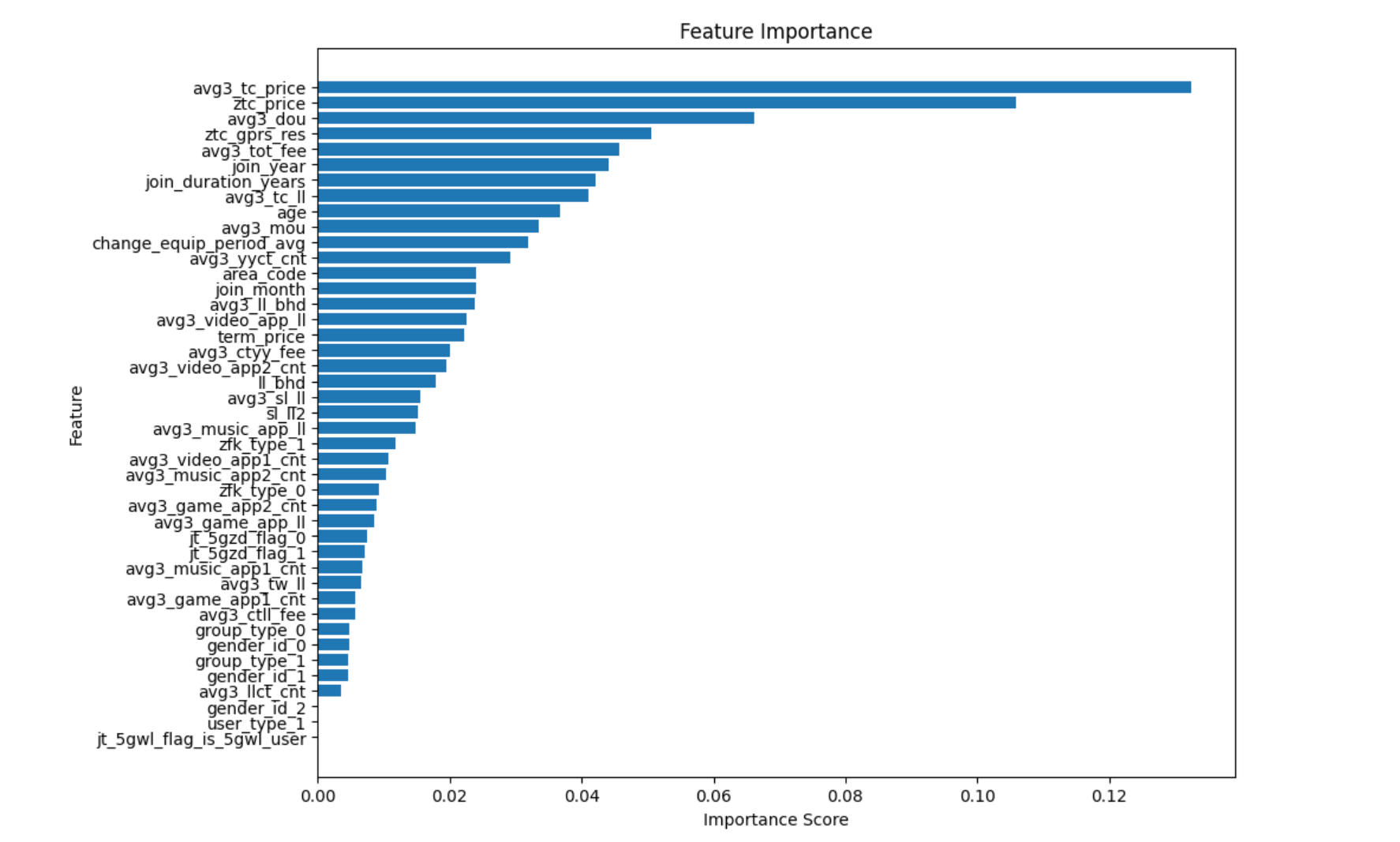
数据集划分（基于前十个重要特征进行训练）

将数据集分为训练集和测试集，确保模型能够在未见过的数据上进行评估。

控制基评估器的参数

参数	含义
criterion	不纯度的衡量指标(基尼系数和信息熵)
n_estimators	树的数量
max_depth	树的最大深度，超过最大深度的树枝都会被剪掉
min_samples_leaf	一个节点在分枝后的每个子节点都必须包含至少min_samples_leaf个训练样本，否则分枝就不会发生
min_samples_split	一个节点必须要包含至少min_samples_split个训练样本，这个节点才允许被分枝，否则分枝就不会发生
max_features	max_features限制分枝时考虑的特征个数，超过限制个数的特征都会被舍弃，默认值为总特征个数开平方取整
min_impurity_decrease	限制信息增益的大小，信息增益小于设定数值的分枝不会发生

import pandas as pd
from sklearn.model_selection import train_test_split, cross_val_score
from sklearn.ensemble import RandomForestClassifier
from sklearn.metrics import accuracy_score, classification_report
from joblib import dump

# 读取预处理后的数据
df_processed = pd.read_csv('/home/workspace/output/toUser/train_processed.csv')

# 选取前10个重要特征
top_10_features = ['avg3_tc_price', 'ztc_price', 'avg3_dou', 'ztc_gprs_res', 'avg3_tot_fee', 
                   'join_year', 'join_duration_years', 'avg3_tc_ll', 'age', 'avg3_mou']

# 分离特征和目标变量
X = df_processed[top_10_features]
y = df_processed['sample_flag']

# 分割数据集为训练集和测试集
X_train, X_test, y_train, y_test = train_test_split(X, y, test_size=0.2, random_state=42)

# 调整随机森林分类器的参数以降低过拟合
rf_model = RandomForestClassifier(
    n_estimators=200,          # 增加树的数量
    max_depth=10,              # 限制树的深度
    min_samples_split=10,      # 内部节点再划分所需的最小样本数
    min_samples_leaf=5,        # 叶节点上的最小样本数
    max_features='sqrt',       # 每次分裂时使用特征的平方根
    random_state=42
)

# 使用交叉验证来评估模型性能
cv_scores = cross_val_score(rf_model, X_train, y_train, cv=5)
print(f"Cross-validation scores: {cv_scores}")
print(f"Mean cross-validation score: {cv_scores.mean()}")

# 训练模型
rf_model.fit(X_train, y_train)

# 预测
y_pred = rf_model.predict(X_test)

# 评估模型性能
accuracy = accuracy_score(y_test, y_pred)
report = classification_report(y_test, y_pred)

print(f"Accuracy: {accuracy}")
print("Classification Report:")
print(report)

# 保存模型
dump(rf_model, '/home/workspace/output/rf_model.joblib')

绘制学习

学习曲线可以展示模型在训练集和验证集上的表现，帮助判断是否存在过拟合或欠拟合的情况。

from sklearn.model_selection import learning_curve
import numpy as np

# 生成学习曲线数据
train_sizes, train_scores, test_scores = learning_curve(rf_model, df_train_preprocessed[top_10_features], target, cv=5)

# 计算均值和标准差
train_scores_mean = np.mean(train_scores, axis=1)
test_scores_mean = np.mean(test_scores, axis=1)

# 绘制学习曲线
plt.figure(figsize=(10, 6))
plt.plot(train_sizes, train_scores_mean, label='Training score', color='blue', marker='o')
plt.plot(train_sizes, test_scores_mean, label='Cross-validation score', color='green', marker='o')
plt.title('Learning Curve')
plt.xlabel('Training examples')
plt.ylabel('Score')
plt.legend(loc='best')
plt.show()

过拟合

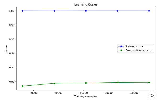
• 训练集表现：
  • 蓝色曲线表示模型在训练集上的表现，接近于 1.0（即接近完美的得分），这表明模型在训练集上拟合得非常好。
  • 这种情况通常说明模型在训练集上几乎没有误差，可能存在过拟合现象。
• 验证集表现：
  • 绿色曲线表示模型在交叉验证集上的表现，得分较低，约在 0.90 左右，且随着训练数据量的增加，该分数并没有显著提升。
  • 这种差距显示模型在验证集上表现不佳，表明模型可能过拟合训练数据，无法很好地泛化到未见的数据。
• 过拟合的迹象：
  • 训练集和验证集的曲线差距较大，且训练集得分过高，这通常是过拟合的典型表现。
  • 模型能够很好地记住训练集的数据，但在验证集上表现欠佳，说明模型可能过于复杂，未能有效学习到数据的泛化特征。

欠拟合

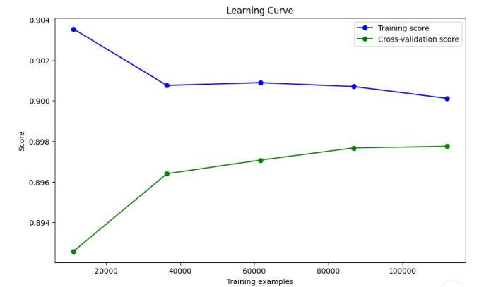
1. 训练分数（蓝线）随着训练样本增加而下降，表明模型的复杂度下降，这是正常的现象。训练集上的分数稍高，意味着模型对训练集的拟合较好，但有逐步降低的趋势。
2. 验证分数（绿线）随着训练样本的增加有所上升，并逐渐趋于稳定，表明模型在验证集上的表现正在提升。

尽管训练和验证曲线之间的差距不算太大，验证分数的表现并没有完全收敛到训练分数的水平。这可能是一个 轻微的欠拟合，但总体表现还可以。这表明模型的复杂度可能不足，或者特征还可以进一步优化。

参数调整对拟合情况的影响总结：

• n_estimators（树的数量）：增加 n_estimators 会提高模型的表现，因为更多的树可以捕捉更多的模式，但增至一定量后会趋于平稳且带来计算开销。200 棵树应该是合理的设置。
• max_depth（树的最大深度）：限制树的深度（如设置为10）可以防止过拟合。如果深度太小，可能导致欠拟合（模型的表现有限）。增加 max_depth 会提高模型复杂度，但也增加过拟合的风险。
• min_samples_split（节点划分的最小样本数）：增大该参数（如设置为10）可以让模型要求更多数据点才能进一步分裂，这样减少了树的复杂度，进而减少过拟合风险。
• min_samples_leaf（叶节点的最小样本数）：设置叶节点的最小样本数为5，可以确保模型不会为了少数样本创建过多的分支，避免过拟合。
• max_features（每次分裂时考虑的最大特征数）：设置 max_features='sqrt' 意味着在每次分裂时考虑一部分随机特征，这通常有助于降低过拟合。这个设置尤其适合高维特征的数据集。

绘制验证曲线

验证曲线可以显示超参数变化时的模型表现，从而帮助你进一步优化超参数。

from sklearn.model_selection import validation_curve

chaocanshu = "max_depth" #超参数

# 生成验证曲线数据
param_range = np.arange(1, 401, 10) # 从A到B，步长为c
train_scores, test_scores = validation_curve(
    RandomForestClassifier(random_state=42),
    X_train, y_train, param_name=chaocanshu, param_range=param_range,
    cv=5, scoring="accuracy", n_jobs=-1)

# 计算训练和验证得分的均值和标准差
train_scores_mean = np.mean(train_scores, axis=1)
test_scores_mean = np.mean(test_scores, axis=1)

# 绘制验证曲线
plt.figure(figsize=(10, 6))
plt.plot(param_range, train_scores_mean, 'o-', color="blue", label="Training score")
plt.plot(param_range, test_scores_mean, 'o-', color="green", label="Cross-validation score")
plt.title(f'Validation Curve for Random Forest ({chaocanshu})')
plt.xlabel(chaocanshu)
plt.ylabel('Score')
plt.legend(loc="best")
plt.grid()
plt.show()

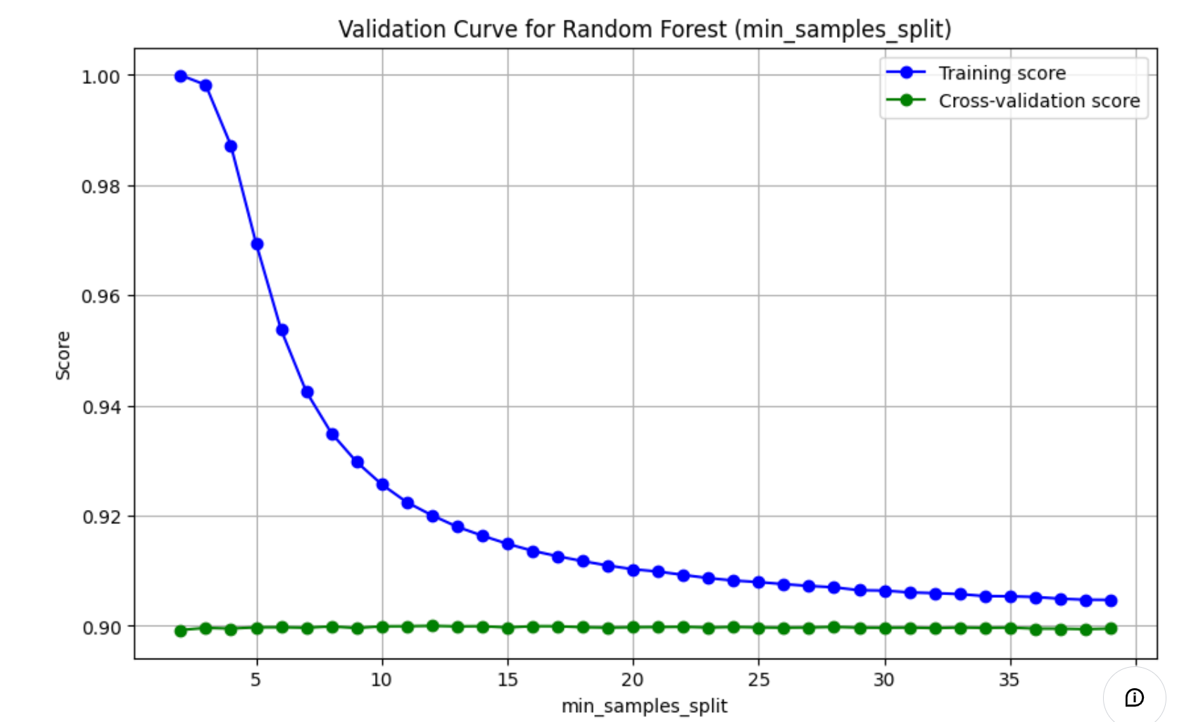
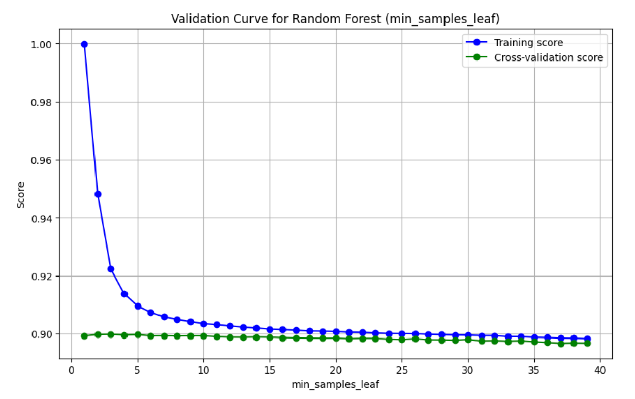
• 训练得分（Training score）：表示模型在训练集上的准确率。随着 max_depth的增加，训练得分可能会先增加后减少，因为模型可能会逐渐适应训练数据，但最终可能会过拟合。
• 交叉验证得分（Cross-validation score）：表示模型在交叉验证集上的准确率。这是一个更可靠的性能指标，因为它考虑了模型在未见过的数据上的表现。
• 曲线的形状：通常，随着 max_depth的增加，模型的复杂度增加，训练得分可能会提高，但交叉验证得分在达到某个点后可能会下降，这表明模型开始过拟合。
• 通过这个验证曲线，你可以找到最佳的 max_depth值，使得模型在训练集和验证集上都能达到较好的性能，从而避免过拟合。

参数选择

1. 找到交叉验证得分最高的点：这是模型在未见过的数据上表现最好的点。
2. 检查过拟合：如果训练得分和交叉验证得分之间的差距很大，这可能意味着过拟合。选择一个差距较小的点以避免过拟合。
3. 考虑实际应用：在实际应用中，你可能需要考虑模型的复杂度和训练时间。较深的树可能需要更长的时间来训练。